App Engine
The process of splitting written text into meaningful components, such as words, sentences, or phrases, is known as text segmentation. Natural language processing refers to both the mental processes that humans utilise when reading text and the artificial processes that are implemented in computers.
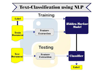
This blog describes how text segmentation can be performed with the help of Hidden Markov model(HMM)
Natural language processing (NLP) challenges are where naive Bayes are most commonly utilised. Naive Bayes predicts a text's tag. They calculate each tag's probability for a given text and output the tag with the highest probability. In Naive Bayes, we calculate the probability of label y using the joint probability, assuming that the input values are conditionally independent. Because letter or word sequences are dependent, this assumption does not hold true in the text segmentation problem.
We present a parameter-free text segmentation approach based on a left-to-right hidden Markov model (HMM) as the text stream's generative model. Each state of the HMM is linked to a certain topic and develops a storey about that topic. The process of fitting HMMs to the input text stream can then be viewed as text segmentation. In other words, text segmentation can be thought of as HMM learning with a text stream as input.
Hidden Markov model(HMM):
Segmenter:
Suppose that there are k topics T(1), T(2), . . . , T(k)). There is a language model associated with each topic T(i),1 <= i <= k, using which one can calculate the probability of any sequence of words. In addition, there are transition probabilities among the topics, including a probability for each topic to transition to itself (the “selfloop” probability), which implicitly specifies an expected duration for that topic. Given a text stream, a probability can be attached to any particular hypothesis about the sequence and segmentation of topics in the following way:
1. Transition from the start state to the first topic and accumulate a transition probability.
2. Stay in topic for a certain number of words or sentences, and, given the current topic, accumulate a self-loop probability and a language model probability for each.
3. Transition to a new topic, accumulate the transition probability, and go back to step two
The Hidden Markov Model provides a joint distribution over the letters/tags with an assumption about the relationships of variables x and y between consecutive tags, as an extension of Naive Bayes for sequential data.
As we know from the naive bayes' model:
HMM puts state transition P(Y_k|Y_k-1). Now we have:
Therefore in HMM, we change from P(Y_k) to P(Y_k|Y_k-1).
This model is a generative technique, similar to Naive Bayes. It models the entire probability of inputs by modelling the joint probability P(X,Y) and then applying the Bayes theorem to obtain P(YX). The emission matrix P(X kY k) is the one we saw earlier. In Naive Bayes, the emission matrix shows the likelihood of a character for a given tag. So here's an example of a matrix of tag and input character joint probability:
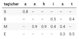
The likelihood of each tag transitioning to an adjacent tag is given by the P(Y k Y k-1) portion. For example, given prior tag (Y k-1) let us say 'S,' the likelihood of current tag (Y k) let us say 'B'.

Fig. Transition matrix
From the graph below, this would be 0.8. A transition matrix is what this is termed. We can think of Naive Bayes joint probability between label and input but independence between each pair in a graph structure. It can be represented as follows:
[B] [M] [M] [E] [B] [E] [S] ...
| | | | | | |
[t] [h] [i] [s] [i] [s] [a] ...
The graph depicts the interdependencies between states for HMM:
[Start]=>[B]=>[M]=>[M]=>[E]=>[B]=>[E]=>[S]...
| | | | | | |
[t] [h] [i] [s] [i] [s] [a]...
Another generic illustration of Naive Bayes and HMM may be found here.

The next step is to determine the optimal sequence.
Viterbi Algorithm:
The Viterbi method, which gives an efficient way of obtaining the most likely state sequence with a maximum probability, is used to determine the best score from all conceivable sequences.
Each node in the trellis below represents a different state for a given sequence. The arrow indicates a probable transition from one condition to the next. The goal is to identify the path that offers us the highest probability by filling out the trellis with all possible values starting at the beginning of the sequence and working our way to the finish.

The calculation in the original technique takes the product of the probabilities, and the result gets very little as the series grows longer (bigger k). At some point, the value will be too small for the floating-point precision, resulting in a calculation that is imprecise. This is referred to as "underflow." Because it is a monotonically growing function, the adjustment is to use a log function.
Experiment:
As a baseline comparison to the CRF comparison in a subsequent post, we employed a Chinese word segmentation implementation on our dataset and got 78 percent accuracy on 100 articles. This technique, unlike prior Naive Bayes implementations, does not employ the same feature as CRF. We also employ the four states depicted above.
Data from 100 articles with a 20% test split on performance training.
799 sentences, 28,287 words in the training set
182 sentences, 7,072 words in the test set
      precision    recall  f1-score   support           0       0.95      0.76      0.84     25107
           1       0.50      0.84      0.63      7072    accuracy                           0.78     32179
   macro avg       0.72      0.80      0.73     32179
weighted avg       0.85      0.78      0.79     32179
Fig. Detail metric
Similar to bigram and trigram, we can have a high order of HMM. First-order HMM, which is similar to bigram, is the current description. We can apply the second-order method, which employs the utilisation of trigrams.
Other Chinese segmentation has a performance range of 83 percent to 89 percent on various datasets.
Puthick Hok observed that the HMM Performance on Khmer manuscripts was 95% accurate with less unknown or mistyped words.
HMM flaws:
HMM is a joint distribution based on the assumption of earlier token independence events. We are not implying that each occurrence is independent of the others, but rather that each label is independent. HMM captures dependencies between each state and just the observations that correspond to it. However, each segmental condition may be influenced not just by a single character/word, but also by all subsequent segmental phases.
In addition, there is a misalignment between the learning objective function and prediction. The objective function of the HMM learns a joint distribution of states and observations P(Y, X), but we need P(Y|X) for prediction tasks.
Conclusion:
The goal of HMM is to recover the data sequence when the next sequence of data cannot be observed immediately and the upcoming data is dependent on the old sequences. HMM is widely utilised in many applications. We were able to successfully apply HMM to text segmentation. We've encountered the viterbi algorithm in the context of Markov information sources and hidden Markov models, where the viterbi path results in a sequence of observed events.

References:
https://ieeexplore.ieee.org/abstract/document/674435/
https://medium.com/@phylypo/nlp-text-segmentation-using-hidden-markov-model-f238743d8 7eb
http://www.cs.columbia.edu › ...PDF Topic Segmentation with an Aspect Hidden Markov Model
https://www.semanticscholar.org › A...An HMM-based text segmentation method using variational Bayes
https://www.scielo.br › cspName segmentation using hidden Markov models and its application ...
Authors: Sara Ahmad, Ayush Patidar, Pradyumna Daware, Ashutosh Jha


Comments
Post a Comment